数学
データの補間や曲線の平均などの数学操作をLabTalkで行う場合のスクリプトのサンプルです。
与えられたXについてデータを補間
pe_mkdir Interp1 path:=aa$;  // プロジェクト内にInterp1というフォルダを作成
pe_cd aa$; // フォルダInterp1を開く

fname$ = system.path.program$ + "Samples\Mathematics\Interpolation.dat";
newbook;
newsheet cols:=4 xy:="XYXY";
impasc;

Range rTime1 = 1; // アクティブシートのcol(1)
Range rData1 = 2; // アクティブシートのcol(2)
Range rTime2 = 3; // col(3)
Range rData2 = 4; // col(4)
// 最初の2列をX、Yデータとして3列目のXに対するYの値をスプライン補間して4列目に出力する
interp1 ix:=rTime2 iy:= rData1 method:= spline ox:=rData2 ;
// 結果をプロット
plotxy iy:=rData1 plot:=200 color:=1;
plotxy iy:=rData2 plot:=200 color:=2 ogl:=1;
以下のサンプルでは、ファイルからインポートされたデータをスプラインで補間し、折れ線グラフを作成します。
// サンプルフォルダからデータをインポート
string fname$ = system.path.program$ + "Samples\Curve Fitting\Exponential Decay.dat";
newbook s:=0;
newsheet cols:=4 xy:="XYYY";
impasc;

// 指定された列を補間
for(i=2;i<5;i++){
interp1xy -r 2 iy:=[ExponentialDe]1!$(i) method:=spline npts:=200;
}

plotxy ((1,5),(1,6),(1,7)) plot:=200; // グラフを作成
曲線を平均
次のサンプルでは、Xが単調に増加する複数のXYデータを平均します。Xは必ずしも共有X値である必要はありません。
/*
サンプルデータのパス:Originインストールフォルダ\Samples\Spectroscopy\DSC\Data folder

1. 同じブック内の異なるワークシートにデータをロード
2. Xファンクションavecurvesを使ってすべてのシートのA(X)B(Y)を平均
3. 結果を新しいシートに出力
4. 元データと平均のデータを別々のグラフとして作図
*/

// サンプルファイルloadDSC.ogsを使ってサンプルデータを異なるシートにロード
string LoadDSCogsPath$=system.path.program$ + "Samples\LabTalk Script Examples\LoadDSC.ogs";
%A=LoadDSCogsPath$;
if(!run.section(%A, Main, 0))
	break 1;
// アクティブシートにデータがロードされる
string dscBook$=%H;
// データA(X), B(Y)でグラフを作成
plotxy [dscBook$](1:end)!(1,2) plot:=200;

// 線形補間平均の手法を使って全シートのデータを平均
avecurves iy:=[dscBook$](1:end)!(1,2) rd:=[<input>]<new name:="Averaged Data">! method:=ave interp:=linear;
// 平均データも作図
plotxy [dscBook$]"Averaged Data"!(1,2) plot:=200 ogl:=[<new>]<new>!;
2D補間
Xファンクションminterp2を使って、行列に2D補間/補外を実行できます。
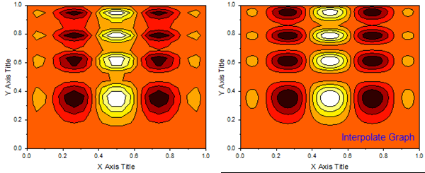
newbook name:=MyMatrix1 mat:=1;

// 行列次数と値をセット
matrix -ps DIM 20 20;
matrix -ps X 0 1;
matrix -ps Y 0 1;
matrix -v x*(1-x)*cos(4*PI*x)*sin(4*PI*y^2)^2;
// スプラインで補間
minterp2 -r 2 im:=<active> cols:=50 rows:=50 xmin:=0 xmax:=1 ymin:=0 ymax:=1 om:=Interp;

// 元の行列データを等高線図として作図
plotm im:=[MyMatrix1]1! plot:=226 ogl:=<Contour>;
layer.cmap.load(Fire.pal,0);
// 結果行列のデータ
plotm im:=[Interp]1! plot:=226 ogl:=[<new>]<new>;
layer.cmap.load(Fire.pal,0);
layer.matmaxptsenabled=0; // スピードモードオフ
ポリゴンの面積
このグラフのようなヒステリシス・ループの場合、以下のスクリプトを使ってポリゴンの面積を計算できます。
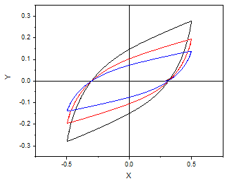
// グラフをアクティブにする
type Dataset     Loop Area;
doc -e d // アクティブグラフウィンドウの全プロットでループ
{
polyarea iy:=%C type:=1;
type %C       $(polyarea.Area,%2.2f);
}

/*結果表
Index     Loop Area
Book1_B      0.23
Book1_C      0.16
Book1_D      0.11
*/
その他のスクリプトサンプル