
サンプルスクリプト
[7-1] レーザーの熱流解析 【Laser_Heaflow.pde】
1. 概要
この問題は、複雑な熱流問題への適用を示します。レーザーロッドは、銅のシリンダー内部に接着されます。製造誤差でロッドは接着剤の内部へ移動します。そして、ロッドまわりの接着剤層が不均一になります。
接着剤は断熱材(熱伝導率=0.0019)で、ロッドからの放熱を妨げます。
銅のシリンダーは、その外表面の60度の角度範囲だけで、冷やされます。
レーザーロッドは、温度に依存した熱伝導率を持ちます。
我々は、レーザーロッドの温度分布を把握したいです。
熱流方程式は div(K*grad(Temp)) + Source = 0.
シリンダーの横断面をモデル化します。
これが円筒形の構造であると同時に、横断面は、暗黙の回転が直交座標平面内なので、方程式は直交座標系です。
半径2mmのロッド内部に、200(W/cc)の熱源があります。
ロッドの熱伝導率:39.8/(300+temp) (W/cm/K),temp:温度
-- この問題は、Luis Zapataによって提出されました。
2. メッシュ図
{Fig.A}~{Fig.E} は、4項で対応するスクリプトを示します。
図示でX,Y軸の単位はcmです。
{Fig.A} に解析領域の全体メッシュ図を示します。
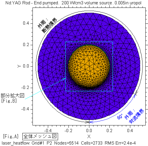
{Fig.A} で
  明るい茶色部分:ロッド(半径2mm) 熱伝導率:39.8/(300+temp) (W/cm/K),temp:温度
  緑色部分   :接着剤層(厚さ 0.05±0.025mm) 熱伝導率=0.0019
  青紫色部分  :銅(半径5mm)   熱伝導率=3.0
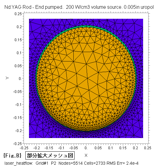
空色枠線部分を拡大して {Fig.B} に示します。ロッドが下方に偏って、接着剤層が上側で厚く、下側で薄くモデル化されていることが分かります。
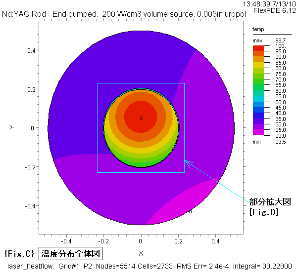
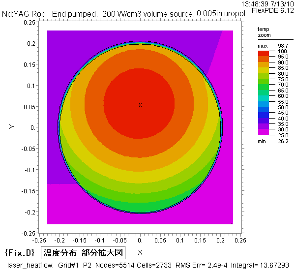
3. 解析結果
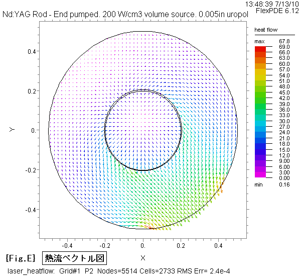
温度分布の全体図を{Fig.C}、部分拡大図を{Fig.D}、熱流のベクトル図を{Fig.E} に示します。
接着剤層の内側と外側で、温度に大きな差が生じています(断熱効果)。
熱流ベクトルの向きが、等温線と直交しています。
断熱境界に沿っては平行で、下側の対流(冷却)境界に対しては垂直な流れが表現されています。
メッシュ精度の問題から完全な平行、垂直ではない部分もあります。
4. スクリプト
下記のスクリプトをマウスでコピーし、FlexPDE エディット・ウィンドウに貼り付けて実行する際は、日本語のコメントを除去して下さい。そのままですと、コンパイル・エラーが発生する場合があります。
{ LASER_HEATFLOW.PDE

This problem shows a complex heatflow application.

A rod laser is glued inside a cylinder of copper.

Manufacturing errors allow the rod to move inside the glue, leaving a non-uniform glue layer around
the rod.
The glue is an insulator, and  traps heat in the rod.  The copper cylinder is cooled only on a
60-degree portion of its outer surface.

The laser rod has a temperature-dependent conductivity.

We wish to find the temperature distribution in the laser rod.

The heat flow equation is

	div(K*grad(Temp)) + Source = 0.

We will model a cross-section of the cylinder. While this is a cylindrical structure, in cross-section
 there is no implied rotation out of the  cartesian plane, so the equations are cartesian.

	-- Submitted by Luis Zapata
}

title "Nd:YAG Rod - End pumped.  200 W/cm3 volume source. 0.005in uropol"

Variables
    temp    { declare "temp" to be the system variable }

definitions
    k = 3               { declare the conductivity parameter for later use 熱伝導率デフォルト値 }
    krod=39.8/(300+temp){ Nonlinear conductivity in the rod.(W/cm/K) ロッドの温度依存性熱伝導
率 }
    Rod=0.2             { cm Rod radius ロッドの半径 cm }
    Qheat=200           { W/cc, heat source in the rod ロッド内の熱源 }

    kuropol=.0019   { Uropol conductivity 接着剤層の熱伝導率 }
    Qu=0            { Volumetric source in the Uropol 接着剤層内の熱源 }
    Ur=0.005        { Uropol annulus thickness in r dim 接着剤層の厚さ cm }

    kcopper=3.0     { Copper conductivity 銅の熱伝導率 }
    Rcu=0.5         { Copper convection surface radius 銅の外周半径 cm }

    tcoolant=0.     { Edge coolant temperature 冷却部の温度 }
    ASE=0.          { ASE heat/area to apply to edge, heat bar or mount }
    source=0

initial values
    temp = 50       { estimate solution for quicker convergence 温度初期値:すばやい収束のため
の推定解 }

equations           { define the heatflow equation 熱流方程式 }
    temp : div(k*grad(temp)) + source = 0;

boundaries
    region 1        { the outer boundary defines the copper region 銅の外周境界 }
        k = kcopper
        start (0,-Rcu)
        natural(temp) = -2 * temp       {convection boundary 対流境界 }
            arc(center=0,0) angle 60
        natural(temp) = 0               {insulated boundary 断熱境界 }
            arc(center=0,0) angle 300
            arc(center=0,0) to close

    region 2
	{ next, overlay the Uropol in a central cylinder 円筒の中心に接着剤層を重ねて定義し
ます→region 1 に上書き }
        k = kuropol
        start (0,-Rod-Ur) arc(center=0,0) angle 360

    region 3	{ next, overlay the rod on a shifted center 中心を -Ur/2 だけずらしてロッドを重ねて定義
します→上書き }
        k = krod
        Source = Qheat
        start (0,-Rod-Ur/2) arc(center=0,-Ur/2) angle 360

monitors
    grid(x,y) zoom(-8*Ur, -(Rod+8*Ur),16*Ur,16*Ur)
    contour(temp)

plots
    grid(x,y)								{Fig.A}
    grid(x,y)	zoom(-(Rod+0.03),-(Rod+0.03),2*(Rod+0.03),2*(Rod+0.03))		{Fig.B}
    contour (temp)	painted						{Fig.C}
    contour(temp)	zoom(-(Rod+0.03),-(Rod+0.03),2*(Rod+0.03),2*(Rod+0.03))	painted
	{Fig.D}
    contour(temp) zoom(-(Rod+Ur)/4,-(Rod+Ur),(Rod+Ur)/2,(Rod+Ur)/2)	painted
    vector(-k*dx(temp),-k*dy(temp)) as "heat flow"				{Fig.E}
    surface(temp)

end