サンプルスクリプト
[9-1] ドーパントの拡散解析 【Diffusion.pde】

1. 概要

この問題は、一定の不純物ソースから固体に熱的に運ばれるドーパント（半導体に添加する微量の不純物）の拡散を考慮します。
半導体拡散で典型的に使用されるパラメータを選びました。
〔　〕内は、[4. スクリプト] 項での設定値です。

表面の集中 = 1.8e20 atoms/cm^2 〔1.8e8 atom/micron^3〕拡散係数     = 3.0e-15cm^2/sec     〔1.1e-3 micron^2/hr〕

この種の問題の自然の傾向は、材料のゼロ集中と境界上の一定値で遮断することです。
これは、境界上の無限大の曲率と、拡散する粒子の無限大の移送速度を意味します。
有限要素法がステップ関数に２次方程式論を当てはめようとするので、解にオーバー･シュートも生み出します。

より良い定式化は、大きな入力流束、ドーパントが実際に境界を横切ることができる率の代表値（または、分子速度が境界上での集中不足の時間をほぼ決定します）をプログラムすることです。

ここでは、２次元パターンを生成するために、我々はマスクした不純物ソースを使います。
これは、結果が後期で解析的平面拡散結果より少し遅れる原因になります。

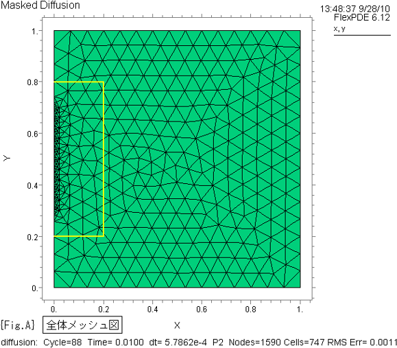
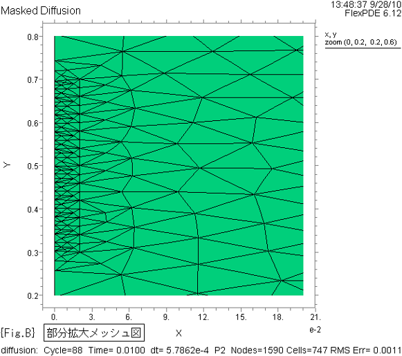
2. メッシュ図

{Fig.A} に解析領域の全体メッシュ図を示します。
{Fig.A} の黄色枠線部分を拡大して {Fig．B} に示します。
{Fig.A}，{Fig.B} は、４項で対応するスクリプトを示します。

 

3. 解析結果

{Fig.C}～{Fig.G} は、４項で対応するスクリプトを示します。
{Fig.C}，{Fig.D} に、ドーパントの拡散状況をそれぞれ２Ｄ等高線図、３Ｄ曲面図で示します。

{Fig.C}，{Fig.D} は、各時間（1e-5, 1e-4, 1e-3, 1e-2, 0.05, 0.1, 0.15, 0.2, 0.3, 0.4, 0.5, 0.6, 0.7, 0.8, 0.9, 1.0）ごとの状態を示す画像ファイルを FlexPDE から出力した後、Jasc Animation Shop 等の市販ソフトでアニメ.gifファイルへ変換して作成しました。

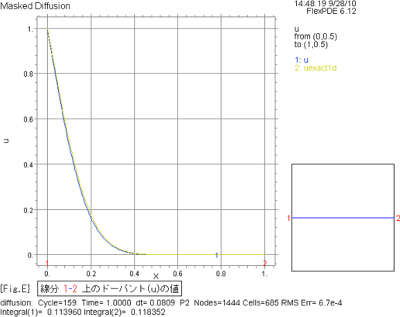
{Fig.E} に、線分1-2上のドーパント(u)の値をグラフで示します。

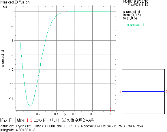
{Fig.F} に、線分1-2上のドーパント(u)の厳密解との差をグラフで示します。
Y軸の目盛は1000倍した数値です。　上方に e-3 と表記しています。

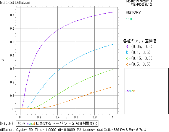
{Fig.G} に、各点におけるドーパント(u)の時間変化グラフを示します。

4. スクリプト

下記のスクリプトをマウスでコピーし、FlexPDE エディット･ウィンドウに貼り付けて実行する際は、日本語のコメントを除去して下さい｡ そのままですと、コンパイル･エラーが発生する場合があります｡

{ DIFFUSION.PDE

  This problem considers the thermally driven diffusion of a dopant into
  a solid from a constant source.  Parameters have been chosen to be those
  typically encountered in semiconductor diffusion.

    surface concentration = 1.8e20 atoms/cm^2
    diffusion coefficient = 3.0e-15 cm^2/sec

  The natural tendency in this type of problem is to close off with zero
  concentration in the material, and a fixed value on the boundary.  This
  implies an infinite curvature at the boundary, and an infinite transport
  velocity of the diffusing particles.  It also generates over-shoot
  in the solution, because the Finite-Element Method tries to fit a step
  function with quadratics.

  A better formulation is to program a large input flux, representative of
  the rate at which dopant can actually cross the boundary, (or approximately
  the molecular velocity times the concentration deficiency at the boundary).

  Here we use a masked source, in order to generate a 2-dimensional pattern.
  This causes the result to lag a bit behind the analytical Plane-diffusion
  result at late times.

}

title
  'Masked Diffusion'

variables
  u(threshold=0.1)

definitions
  concs = 1.8e8             { surface concentration  atoms/micron^3　面の集中 }
  D = 1.1e-2                { diffusivity micron^2/hr　拡散係数 }
  conc = concs*u
  cexact1d = concs*erfc(x/(2*sqrt(D*t)))
  uexact1d = erfc(x/(2*sqrt(D*t)))	{ u の厳密解 }
                            { masked surface flux multiplier　マスクした面流束の乗数 }
  M = 10*upulse(y-0.3,y-0.7)

initial values
  u = 0

equations
  u : div(D*grad(u)) = dt(u)

boundaries
  region 1
    start(0,0)
    natural(u) = 0      line to (1,0)
    natural(u) = 0      line to (1,1)
    natural(u) = 0      line to (0,1)
    natural(u) = M*(1-u)  line to close

  feature               { a "gridding feature" to help localize the activity　不純物ソース、及びメッシュ細分化の
範囲を限定します }
    start (0.02,0.3) line to (0.02,0.7)

time 0 to 1 by 0.001

plots
  for t=1e-5 1e-4 1e-3 1e-2 0.05 by 0.05 to 0.2 by 0.1 to endtime
{ Time=1e-5, 1e-4, 1e-3, 1e-2, 0.05, 0.1, 0.15, 0.2, 0.3, 0.4, 0.5, 0.6, 0.7, 0.8, 0.9, 1.0 について以下を
出力します }
    grid(x, y)						{Fig.A}
    grid(x, y)	zoom (0, 0.2,  0.2, 0.6)		{Fig.B}
    contour(u)						{Fig.C}
    surface(u)						{Fig.D}
    elevation(u,uexact1d) from (0,0.5) to (1,0.5)	{Fig.E}
    elevation(u-uexact1d) from (0,0.5) to (1,0.5)	{Fig.F}

histories
  history(u) at (0.05,0.5) (0.1,0.5) (0.15,0.5) (0.2,0.5)   {Fig.G}

end