サンプルスクリプト
[6-1]] 3D熱伝導解析 【3D_Bricks.pde】

1. 概要

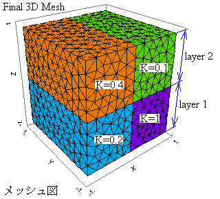
３Ｄ 定常熱伝導解析の例です。それぞれ異なる４種類の熱伝導率（K）を持つ直方体の集合体内部に、ガウス形分布の熱源があります。全ての表面（６面）は、０度に保持されています。　一定の時間が経過しますと、温度は安定した分布状態に到達します。本サンプルは、3D_Bricks+Time.pdeの定常状態に類似しています。

2. メッシュ図

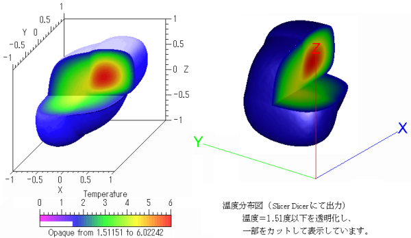
3. 解析結果

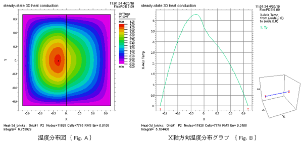
図中の {Fig.A}，{Fig.B} は、４項で対応するスクリプトを示します。

4. スクリプト

下記のスクリプトをマウスでコピーし、FlexPDE エディット･ウィンドウに貼り付けて実行する際には、日本語のコメントを除去して下さい。そのままですと、コンパイル･エラーが発生する場合があります｡

{ 3D_brICKS.PDE

 This problem demonstrates the application of FlexPDE to steady-state
 three dimensional heat conduction.  An assembly of four bricks of
 differing conductivities has a gaussian internal heat  source,  with all
 faces held at zero temperature.  After a time, the  temperature reaches
 a stable distribution.

 This is the steady-state analog of problem 3D_brICKS+TIME.PDE
}

title 'steady-state 3D heat conduction'

select
    regrid=off  { use fixed grid }
    painted	{ 等高線図を色分けで塗りつぶします。}

coordinates
    cartesian3

variables
    Tp		{ 温度 }

definitions
    long = 1
    wide = 1
    K   { thermal conductivity -- values supplied later　熱伝導率：値は後で設定します。}
    Q = 10*exp(-x^2-y^2-z^2)    { Thermal source　ガウス形分布の熱源 }

initial values
    Tp = 0.

equations
    Tp : div(k*grad(Tp)) + Q = 0    { the heat equation }

extrusion z = -long,0,long      { divide Z into two layers　Ｚ軸を２つのlayerに分割します。}

boundaries
    Surface 1 value(Tp)=0       { fix bottom surface temp }
    Surface 3 value(Tp)=0       { fix top surface temp }

    Region 1    { define full domain boundary in base plane }
       layer 1 k=1              { bottom right brick }
       layer 2 k=0.1            { top right brick }
       start(-wide,-wide)
         value(Tp) = 0          { fix all side temps }
         line to (wide,-wide)   { walk outer boundary in base plane }
           to (wide,wide)
           to (-wide,wide)
           to close

    Region 2    { overlay a second region in left half }
       layer 1 k=0.2            { bottom left brick }
       layer 2 k=0.4            { top left brick }
       start(-wide,-wide)
         line to (0,-wide)      { walk left half boundary in base plane }
           to (0,wide)
           to (-wide,wide)
           to close

monitors
    contour(Tp) on z=0  as "XY Temp"
    contour(Tp) on x=0  as "YZ Temp"
    contour(Tp) on y=0  as "ZX Temp"
    elevation(Tp) from (-wide,0,0) to (wide,0,0)  as "X-Axis Temp"
    elevation(Tp) from (0,-wide,0) to (0,wide,0)  as "Y-Axis Temp"
    elevation(Tp) from (0,0,-long) to (0,0,long)  as "Z-Axis Temp"

plots
	cdf(Tp)
    contour(Tp) on z=0  as "XY Temp"					{ Fig.A }
    contour(Tp) on x=0  as "YZ Temp"
    contour(Tp) on y=0  as "ZX Temp"
    elevation(Tp) from (-wide,0,0) to (wide,0,0)  as "X-Axis Temp"	{ Fig.B }
    elevation(Tp) from (0,-wide,0) to (0,wide,0)  as "Y-Axis Temp"
    elevation(Tp) from (0,0,-long) to (0,0,long)  as "Z-Axis Temp"

end